Herding cats is hard. These cowboys herding cats can attest. Have you ever tried to herd elements of correlation matrices? Stan implements a lot of nice functionality to make your correlated life easier and recommends the LKJ correlation distribution and correlation matrix transform but this 3 part post is about herding cats not shooting fish in a barrel. This post is about rolling your own correlation matrix, if you need to.
Well known problem
On the Stan forums you’ll find a post every so often (see here, here, here) detailing issues with large correlation matrices. The general advice by Ben Goodrich on this post is worth repeating here,
Any moderate sized covariance matrix has a good chance to become numerically problematic for some values of the structural parameters that Stan lands on during the leapfrom process. Basically, the advice is
- Parameterize things in terms of a Cholesky factor of a covariance matrix when possible
- If the error is due to numerical asymmetry, you can do something like R = 0.5 * (R + transpose(R)) after filling it.
- If the error is due to numerical indefiniteness, you can add a tiny positive constant to the diagonal of R after filling it or do something more complicated.
Ok, so just use Cholesky factors, make sure it’s symmetric, and add some positive noise to the diagonal. That doesn’t seem too hard. Sometimes you have additional information that constrains the correlation matrix to block structure, Toeplitz, or you just have a really big correlation matrix and the Stan LKJ isn’t working well. This post is for you. It’s not an exhaustive treatment of correlation matrices but it’s meant to gather some information that’s located on the forums and elsewhere to showcase a couple of alternative parameterizations.
Correlation Crazies
A correlation matrix must satisfy a few conditions
- 1s on the diagonal.
- Off diagonal elements are bound between [−1,1].
- It’s positive-semidefinite.
The third point is the difficulty. Even in 3-dimensions the space is pretty constrained. I got the idea of creating the below gif from Rick Wilkin’s post on the SAS blog. It is the valid space of triplets for a 3 × 3 correlation matrix. The matrix determinant must be,

This valid space looks like a samosa floating around the [-1, 1] cube,

You can also see Ben’s post about how the volume of the sample space decreases as the dimension of the correlation matrix increases. Showing the constant of integration for the distribution by varying sizes of K,
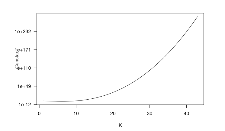
which means that the space decreases super fast, on the order of 
Ulterior Correlations
The LKJ distribution is nice and has good computational qualities that make it an excellent choice for many problems. That may not work for your problem so this post is for you.
Searching around I’ve found that everyone and their mom seems to have tried their hand at this probelm. There are many different parameterizations. Here are a few I found that you may be interested in (let me know in the comments if you know of any others):
- Onion method
- Matrix F distribution
- Gaussian Inverse Wishart
- Using the boundaries of correlations
- Matrix logarithm
I’m going to focus on method 4 and show a an example of when you may want to do something like this.
Lastly, if you have time in between posts, check out the paper Pinheiro and Bates (1996) on different parameterizations of correlation matrices as methods 4 – 5 stem from those.
Hard Model to Estimate: Non-zero Block Correlation Structure
This blog post came about because I’m working on a problem that has natural block correlation structure. LKJ is not for this problem. Though it will be interesting to see how it performs as a base comparison.
The first step is to simulate a block correlation structure. Umm…
That’s not so easy because our problem largely stems from not easily generating a PSD matrix. Lucky for you, I spent some time coding up something that does just that modifying the method in Numpacharoen and Atsawarungruangkit (2012). They have Matlab code that I followed, adapted to R, then changed to get the block structure I wanted. The elements within blocks are allowed to vary, there’s correlation across blocks, but this is constant for the elements across the two blocks of interest.
The correlation matrix will look as follows,
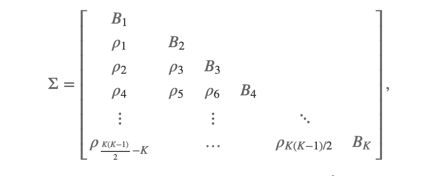
with each 


My modified method is below. I encourage you to read the paper as the method essentially parameterizes the correlation matrix in spherical coordinates (as in Pinheiro and Bates (1996)). The benefit is that we can get out the Cholesky factor without doing the Cholesky decomposition on the generated correlation matrix. I left out randomly permuting the rows-columns because I didn’t want to do all the accounting work to get the right Cholesky factor.
The function takes in the parameters n, threshold, block_size, sigma, sigma_off.
#' Generate a positive-definite block correlation matrix.
#'
#' The sigma size results in the size of the correlations. Adapted from
#' the Matlab code by Kawee Numpacharoen and method in
#'   Reference: Numpacharoen, K. and Atsawarungruangkit, A.,
#'   Generating random correlation matrices based on the boundaries of their coefficients
#'   (August 24, 2012). Available at SSRN: http://ssrn.com/abstract=2127689
#'
#' Copyright (c) 2012, Kawee Numpacharoen and Amporn Atsawarungruangkit, All rights reserved.
#' Copyright (c) 2020, Sean Pinkney, All rights reserved.
#' @param n The size of the correlation matrix.
#' @param threshold The threshold for numerical stability.
#' @param block_size The size of the block. Must be a divisor of n.
#' @param block_idx Identifies the elements within and out of the blocks.
#' @param sigma Positive real.
#' @param sigma_off Positive real.
#' @return A list with the correlation matrix C and Cholesky factor of the correlation matrix B.
#' @export
random_block_cor_nonzero_r <- function(n, threshold, block_size, block_idx, sigma, sigma_off = NULL) {
  num_blocks <- n / block_size
  Bmat <- matrix(0, nrow = n, ncol = n)
  Cmat <- Bmat
  if (is.null(sigma_off)) sigma_off <- sigma / 10
  p <- -1
  while (p < 0){

    Cmat[2:block_size, 1] <- -1 + 2 / (exp( -rnorm(block_size - 1, mean = 0, sd = sigma)) + 1)
    Cmat[(block_size + 1):n] <- rep(-1 + 2 / (exp( -rnorm(num_blocks - 1, mean = 0, sd = sigma_off)) + 1),
                                    each = block_size)
    Bmat[2:n, 1] <- Cmat[2:n, 1]

    for (i in 2:n)
      Bmat[i, 2:i] <- sqrt(1 - Cmat[i, 1] ^ 2)

    temp_matB <- matrix(0, nrow = n, ncol = n)
    for (s in 2:num_blocks){
      for (r in 2:s){
        off_ <- -1 + 2 / (exp( -rnorm(1, mean = 0, sd = sigma_off)) + 1)
        temp_matB[(1 + (s - 1) * block_size):(s * block_size),
                  (1 + (r - 2) * block_size):((r - 1) * block_size)] <- off_
      }
    }

    for (i in 3:n) {
      for (j in 2:(i - 1)) {
        B1 <- Bmat[j, 1:(j - 1)] %*% Bmat[i, 1:(j - 1)]
        B2 <- Bmat[j, j] * Bmat[i, j]
        Z <- B1 + B2 # upper bound
        Y <- B1 - B2 # lower bound

        if (B2 < threshold) {
          Cmat[i, j] <- B1
          cosinv <- 0
        } else if (temp_matB[i, j] != 0){
          if (j <= block_size) Cmat[i, j] <- Cmat[i, 1]
          else Cmat[i, j] <- temp_matB[i, j]
        } else Cmat[i, j] = Y + (Z - Y) *  (1/ (exp( -rnorm(1, mean = 0, sd = sigma)) + 1))

        cosinv <- (Cmat[i, j] - B1) / B2

        if (is.finite(cosinv) == FALSE) {

        } else if (cosinv > 1) {
          Bmat[i, (j + 1):n] <- 0
        } else if (cosinv < -1) {
          Bmat[i, j] <- -Bmat[i, j]
          Bmat[i, (j + 1):n] <- 0
        } else {
          Bmat[i, j] = Bmat[i, j] * cosinv
          sinTheta <- sqrt(1 - cosinv ^ 2)
          for (k in (j + 1):n)
            Bmat[i, k] = Bmat[i, k] * sinTheta
        }
      }
    }
    temp <- Cmat + t(Cmat) + diag(n)
    p <- min(eigen(temp)$values);
  }
  Cmat <- Cmat + t(Cmat) + diag(n)
  Bmat[1, 1] <- 1
  return(list(C = Cmat, B = Bmat))
}
In fact, this method generates the within block correlations according to a normal distribution with mean zero and given sigma. Similarly, the off block correlations are nearly distributed as mean zero and given sigma_off but with more density toward zero. The random normal is transformed with a hyperbolic tangent so that the values are all within [-1, 1].
We are going to work on a correlation matrix size 16 with blocks size 4. I’ll generate the within block correlations with 

block_size = 4
n <- 16
num_blocks <- n / block_size
little_block <- matrix(1, nrow = block_size, ncol = block_size)
little_block[upper.tri(little_block)] <- 0
block_idx <- kronecker(diag(n/block_size), little_block)
block_idx[block_idx == 0] <- 0.0001
block_idx[1, 1] <- 0
sigma <- 1

# seed set in global options for
# rmarkdown to set.seed(2384239)
out <- random_block_cor_nonzero_r(n = n,
                           threshold = 0.001,
                           block_size = block_size,
                           block_idx = block_idx,
                           sigma = 0.5,
                           sigma_off = 0.3)

# Correlation matrix
round(out$C, 2)
       [,1]  [,2]  [,3]  [,4]  [,5]  [,6]  [,7]  [,8]  [,9] [,10] [,11] [,12] [,13] [,14] [,15] [,16]
 [1,]  1.00 -0.45  0.05  0.18 -0.07 -0.07 -0.07 -0.07 -0.04 -0.04 -0.04 -0.04  0.07  0.07  0.07  0.07
 [2,] -0.45  1.00 -0.41  0.04 -0.07 -0.07 -0.07 -0.07 -0.04 -0.04 -0.04 -0.04  0.07  0.07  0.07  0.07
 [3,]  0.05 -0.41  1.00 -0.12 -0.07 -0.07 -0.07 -0.07 -0.04 -0.04 -0.04 -0.04  0.07  0.07  0.07  0.07
 [4,]  0.18  0.04 -0.12  1.00 -0.07 -0.07 -0.07 -0.07 -0.04 -0.04 -0.04 -0.04  0.07  0.07  0.07  0.07
 [5,] -0.07 -0.07 -0.07 -0.07  1.00 -0.05  0.22  0.37  0.08  0.08  0.08  0.08 -0.31 -0.31 -0.31 -0.31
 [6,] -0.07 -0.07 -0.07 -0.07 -0.05  1.00 -0.04  0.20  0.08  0.08  0.08  0.08 -0.31 -0.31 -0.31 -0.31
 [7,] -0.07 -0.07 -0.07 -0.07  0.22 -0.04  1.00 -0.15  0.08  0.08  0.08  0.08 -0.31 -0.31 -0.31 -0.31
 [8,] -0.07 -0.07 -0.07 -0.07  0.37  0.20 -0.15  1.00  0.08  0.08  0.08  0.08 -0.31 -0.31 -0.31 -0.31
 [9,] -0.04 -0.04 -0.04 -0.04  0.08  0.08  0.08  0.08  1.00  0.12 -0.20 -0.05  0.09  0.09  0.09  0.09
[10,] -0.04 -0.04 -0.04 -0.04  0.08  0.08  0.08  0.08  0.12  1.00 -0.35  0.14  0.09  0.09  0.09  0.09
[11,] -0.04 -0.04 -0.04 -0.04  0.08  0.08  0.08  0.08 -0.20 -0.35  1.00  0.09  0.09  0.09  0.09  0.09
[12,] -0.04 -0.04 -0.04 -0.04  0.08  0.08  0.08  0.08 -0.05  0.14  0.09  1.00  0.09  0.09  0.09  0.09
[13,]  0.07  0.07  0.07  0.07 -0.31 -0.31 -0.31 -0.31  0.09  0.09  0.09  0.09  1.00  0.36  0.55  0.38
[14,]  0.07  0.07  0.07  0.07 -0.31 -0.31 -0.31 -0.31  0.09  0.09  0.09  0.09  0.36  1.00  0.40  0.46
[15,]  0.07  0.07  0.07  0.07 -0.31 -0.31 -0.31 -0.31  0.09  0.09  0.09  0.09  0.55  0.40  1.00  0.37
[16,]  0.07  0.07  0.07  0.07 -0.31 -0.31 -0.31 -0.31  0.09  0.09  0.09  0.09  0.38  0.46  0.37  1.00
# Cholesky factor matrix
round(out$B, 2)
       [,1]  [,2]  [,3]  [,4]  [,5]  [,6]  [,7]  [,8]  [,9] [,10] [,11] [,12] [,13] [,14] [,15] [,16]
 [1,]  1.00  0.00  0.00  0.00  0.00  0.00  0.00  0.00  0.00  0.00  0.00  0.00  0.00  0.00  0.00   0.0
 [2,] -0.45  0.89  0.00  0.00  0.00  0.00  0.00  0.00  0.00  0.00  0.00  0.00  0.00  0.00  0.00   0.0
 [3,]  0.05 -0.43  0.90  0.00  0.00  0.00  0.00  0.00  0.00  0.00  0.00  0.00  0.00  0.00  0.00   0.0
 [4,]  0.18  0.13 -0.07  0.97  0.00  0.00  0.00  0.00  0.00  0.00  0.00  0.00  0.00  0.00  0.00   0.0
 [5,] -0.07 -0.12 -0.13 -0.05  0.98  0.00  0.00  0.00  0.00  0.00  0.00  0.00  0.00  0.00  0.00   0.0
 [6,] -0.07 -0.12 -0.13 -0.05 -0.09  0.98  0.00  0.00  0.00  0.00  0.00  0.00  0.00  0.00  0.00   0.0
 [7,] -0.07 -0.12 -0.13 -0.05  0.19 -0.06  0.96  0.00  0.00  0.00  0.00  0.00  0.00  0.00  0.00   0.0
 [8,] -0.07 -0.12 -0.13 -0.05  0.34  0.20 -0.25  0.86  0.00  0.00  0.00  0.00  0.00  0.00  0.00   0.0
 [9,] -0.04 -0.06 -0.07 -0.03  0.06  0.07  0.06  0.05  0.99  0.00  0.00  0.00  0.00  0.00  0.00   0.0
[10,] -0.04 -0.06 -0.07 -0.03  0.06  0.07  0.06  0.05  0.10  0.98  0.00  0.00  0.00  0.00  0.00   0.0
[11,] -0.04 -0.06 -0.07 -0.03  0.06  0.07  0.06  0.05 -0.22 -0.35  0.89  0.00  0.00  0.00  0.00   0.0
[12,] -0.04 -0.06 -0.07 -0.03  0.06  0.07  0.06  0.05 -0.07  0.12  0.11  0.97  0.00  0.00  0.00   0.0
[13,]  0.07  0.12  0.13  0.05 -0.27 -0.30 -0.24 -0.21  0.18  0.16  0.30  0.14  0.73  0.00  0.00   0.0
[14,]  0.07  0.12  0.13  0.05 -0.27 -0.30 -0.24 -0.21  0.18  0.16  0.30  0.14 -0.15  0.71  0.00   0.0
[15,]  0.07  0.12  0.13  0.05 -0.27 -0.30 -0.24 -0.21  0.18  0.16  0.30  0.14  0.10 -0.07  0.72   0.0
[16,]  0.07  0.12  0.13  0.05 -0.27 -0.30 -0.24 -0.21  0.18  0.16  0.30  0.14 -0.13 -0.04 -0.14   0.7
Let’s verify that the created Cholesky matrix when multiplied by itself is equal (within tolerance) to the full correlation matrix,
all.equal(tcrossprod(out$B), out$C)
[1] TRUE
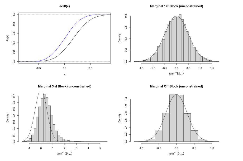
I’ll generate 10000 of these block correlation matrices and plot the marginal distribution to validate my assertion that the marginals are indeed distributed according to our sigmas,
c <- vector(mode = "numeric")
c_later <- vector(mode = "numeric")
c_block <- vector(mode = "numeric")
for (i in 1:10000){
   temp_out <- random_block_cor_nonzero_r(n = n,
                                     threshold = 0.001,
                                     block_size = block_size,
                                     block_idx = block_idx,
                                     sigma = 0.5,
                                     sigma_off = 0.3)
  c[i] <- temp_out$C[1, 2]
  c_later[i] <- temp_out$C[10, 9]
  c_block[i] <- temp_out$C[15, 5]
}
The empirical CDF of the 


Simulate Data
With our correlation matrix in hand let’s generate some values from a multivariate normal with the given correlation matrix.
set.seed(123410)
y <- mvtnorm::rmvnorm(200, sigma = out$C)
Using the LKJ we need to specify 
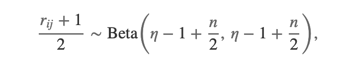
where 


I want to help the LKJ fit as much as possible so I need to get a value of
library(fitdistrplus)
require(MASS)
set.seed(1)
best_shape <- fitdist((c + 1) / 2, "beta", method = "mle")
best_shape
Fitting of the distribution ' beta ' by maximum likelihood
Parameters:
       estimate Std. Error
shape1 8.725937  0.1217450
shape2 8.565027  0.1194353
eta_raw <- mean(best_shape$estimate)

n <- 16
eta <- eta_raw + 1 - n / 2
eta
[1] 1.645482
I solved for
The plot of the fit,

I don’t expect the LKJ model to equal or even perform that well. Let’s get a sense of how “close” the two matrices are. I’ll include in the Stan code a measure of distance from our true correlation matrix to the estimated one. Wu et al. (2018) have a generalized cosine measure they use to test if two correlation (or covariance) matrices are equal. They have four flavors to choose and then construct a permutation test. I’ll just output the one-sample statistic of each of the 4 flavors to get a sense of how our different methods are doing compared to each other. If the metric equals 1 then the two matrices are exactly equal. I’ll code it in Stan so that we get the variance of the statistics for “free”, without having to do anything else in R.
functions {
vector lower_elements(matrix M, int tri_size){
    int n = rows(M);
    int counter = 1;
    vector[tri_size] out;

    for (i in 2:n){
      for (j in 1:(i - 1)) {
        out[counter] = M[i, j];
        counter += 1;
      }
    }
    return out;
  }

  vector gen_cosine(matrix A, matrix B) {
    int n = rows(A);
    int lower_tri_size = n * (n - 1) / 2;
    vector[lower_tri_size] L_A_vech = lower_elements(cholesky_decompose(A), lower_tri_size);
    vector[lower_tri_size] L_B_vech = lower_elements(cholesky_decompose(B), lower_tri_size);
    vector[n] v_A = eigenvalues_sym(A);
    vector[n] v_B = eigenvalues_sym(B);
    vector[n] A_vech = lower_elements(A, lower_tri_size);
    vector[n] B_vech = lower_elements(B, lower_tri_size);
    vector[4] cases; // 4 cases in the paper

    cases[1] = sum( diagonal( A' * B) ) / ( sqrt( sum ( diagonal( crossprod( A ) ) ) ) * sqrt( sum ( diagonal ( crossprod( B ) ) ) ) );
    cases[2] = ( L_A_vech' * L_B_vech ) / ( sqrt( dot_self( L_A_vech ) ) * sqrt( dot_self( L_B_vech ) ) );
    cases[3] = ( v_A' * v_B) / (sqrt( dot_self( v_A ) ) * sqrt( dot_self( v_B ) ) );
    cases[4] = ( A_vech' * B_vech ) / ( sqrt( dot_self( A_vech ) ) * sqrt( dot_self( B_vech ) ) );

    return cases;
  }
}
data {
    int N;
    int cor_size;
    vector[cor_size] y[N];
    matrix[cor_size, cor_size] Sigma_pop;
    real eta;
}
transformed data {
  vector[cor_size] mu = rep_vector(0.0, cor_size);
  vector[cor_size] L_sigma = rep_vector(1.0, cor_size);
}
parameters {
  cholesky_factor_corr[cor_size] L;
}
model {
 L ~ lkj_corr_cholesky(eta);
 y ~ multi_normal_cholesky(mu, diag_pre_multiply(L_sigma, L));
}
generated quantities {
  matrix[cor_size, cor_size] Sigma = multiply_lower_tri_self_transpose(L);
  vector[4] corr_test = gen_cosine(Sigma, Sigma_pop);
}
I created the cosine measure function and a helper function to get the lower triangular elements from the matrix. I’m passing the original correlation matrix to compare to the estimated one in generated quantities. The Cholesky form of the multivariate normal is used and I pass the estimated
stan_data <- list(
  N = 200,
  cor_size = 16,
  y = y,
  block_size = 4,
  block_idx = block_idx,
  Sigma_pop = out$C,
  eta = eta
)

lkj_output <- mod_lkj$sample(data = stan_data,
                      chains = 2,
                      adapt_delta = 0.8,
                      parallel_chains = 2,
                      refresh = 2000
)
Running MCMC with 2 parallel chains...

Chain 1 Iteration:    1 / 2000 [  0%]  (Warmup)
Chain 2 Iteration:    1 / 2000 [  0%]  (Warmup)
Chain 2 Iteration: 1001 / 2000 [ 50%]  (Sampling)
Chain 1 Iteration: 1001 / 2000 [ 50%]  (Sampling)
Chain 2 Iteration: 2000 / 2000 [100%]  (Sampling)
Chain 2 finished in 10.8 seconds.
Chain 1 Iteration: 2000 / 2000 [100%]  (Sampling)
Chain 1 finished in 10.9 seconds.

Both chains finished successfully.
Mean chain execution time: 10.9 seconds.
Total execution time: 11.1 seconds.
No warnings issued, that’s a good sign.
lkj_output$summary("corr_test")
# A tibble: 4 x 10
  variable      mean median      sd     mad    q5   q95  rhat ess_bulk ess_tail
  <chr>        <dbl>  <dbl>   <dbl>   <dbl> <dbl> <dbl> <dbl>    <dbl>    <dbl>
1 corr_test[1] 0.958  0.959 0.00640 0.00667 0.947 0.968  1.00    1682.    1620.
2 corr_test[2] 0.867  0.868 0.0162  0.0163  0.841 0.894  1.00    1464.    1498.
3 corr_test[3] 0.994  0.994 0.00258 0.00249 0.989 0.998  1.00    1549.    1331.
4 corr_test[4] 0.871  0.872 0.0208  0.0215  0.835 0.903  1.00    1753.    1538.
lkj_Sigma <- matrix(lkj_output$summary("Sigma")$mean, ncol = 16)
round(lkj_Sigma, 3)
        [,1]   [,2]   [,3]   [,4]   [,5]   [,6]   [,7]   [,8]   [,9]  [,10]  [,11]  [,12]  [,13]  [,14]  [,15]  [,16]
 [1,]  1.000 -0.495 -0.051  0.234 -0.073 -0.055 -0.059 -0.031 -0.019 -0.061  0.040  0.033  0.077  0.030  0.150  0.010
 [2,] -0.495  1.000 -0.364  0.020 -0.011  0.052 -0.139 -0.020 -0.038 -0.032 -0.018  0.061  0.065  0.008  0.019  0.044
 [3,] -0.051 -0.364  1.000 -0.147 -0.067 -0.086 -0.047 -0.035  0.002 -0.093 -0.066 -0.144  0.010  0.148 -0.017  0.055
 [4,]  0.234  0.020 -0.147  1.000  0.005 -0.128  0.003 -0.070 -0.078 -0.022 -0.029  0.028  0.081 -0.046  0.103  0.037
 [5,] -0.073 -0.011 -0.067  0.005  1.000 -0.063  0.115  0.431  0.143  0.154  0.122  0.060 -0.240 -0.116 -0.223 -0.272
 [6,] -0.055  0.052 -0.086 -0.128 -0.063  1.000 -0.050  0.078  0.020  0.093  0.014  0.066 -0.347 -0.324 -0.274 -0.335
 [7,] -0.059 -0.139 -0.047  0.003  0.115 -0.050  1.000 -0.146  0.022  0.110  0.061  0.020 -0.236 -0.255 -0.268 -0.304
 [8,] -0.031 -0.020 -0.035 -0.070  0.431  0.078 -0.146  1.000  0.130  0.071  0.076  0.081 -0.240 -0.202 -0.252 -0.219
 [9,] -0.019 -0.038  0.002 -0.078  0.143  0.020  0.022  0.130  1.000  0.146 -0.246  0.046  0.173  0.110  0.162  0.012
[10,] -0.061 -0.032 -0.093 -0.022  0.154  0.093  0.110  0.071  0.146  1.000 -0.354 -0.031 -0.006  0.085  0.009  0.027
[11,]  0.040 -0.018 -0.066 -0.029  0.122  0.014  0.061  0.076 -0.246 -0.354  1.000  0.133  0.125  0.042  0.125  0.165
[12,]  0.033  0.061 -0.144  0.028  0.060  0.066  0.020  0.081  0.046 -0.031  0.133  1.000  0.136 -0.036  0.128  0.141
[13,]  0.077  0.065  0.010  0.081 -0.240 -0.347 -0.236 -0.240  0.173 -0.006  0.125  0.136  1.000  0.235  0.484  0.320
[14,]  0.030  0.008  0.148 -0.046 -0.116 -0.324 -0.255 -0.202  0.110  0.085  0.042 -0.036  0.235  1.000  0.205  0.314
[15,]  0.150  0.019 -0.017  0.103 -0.223 -0.274 -0.268 -0.252  0.162  0.009  0.125  0.128  0.484  0.205  1.000  0.413
[16,]  0.010  0.044  0.055  0.037 -0.272 -0.335 -0.304 -0.219  0.012  0.027  0.165  0.141  0.320  0.314  0.413  1.000
The correlation measures show that it fits really nicely. This may not always be the case. We’re Bayesians or Bayes-curious and we should always try to incorporate additional information when we have it. Knowing – or believing – that there is a block structure to the correlation matrix means that we should be able to do better than assuming not. In my next post I’ll show how to roll your own correlation matrix and how this can help estimating these types of problems.
Disclaimer
All views expressed in this post are my own and do not represent the opinions of any entity whatsoever from which I have been, am now, or will be affiliated.
References
Numpacharoen, Kawee, and Amporn Atsawarungruangkit. 2012. “Generating Correlation Matrices Based on the Boundaries of Their Coefficients.” PloS One 7 (November): e48902. https://doi.org/10.1371/journal.pone.0048902.
Pinheiro, José C, and Douglas M Bates. 1996. “Unconstrained Parametrizations for Variance-Covariance Matrices.” Statistics and Computing 6 (3): 289–96.
Wu, Longyang, Chengguo Weng, Xu Wang, Kesheng Wang, and Xuefeng Liu. 2018. “Test of Covariance and Correlation Matrices,” December.

Very nice! Looking forward to the next posts in this series!
LikeLiked by 1 person